Introduction#
Previously, I introduced BitNetMCU, my vehicle for exploring ultra-low-bit quantized neural networks aimed at low-end microcontrollers.
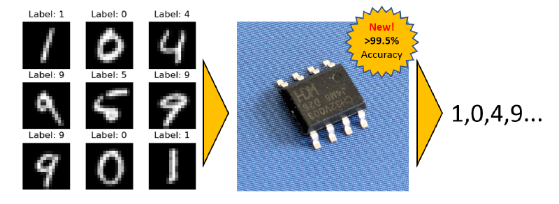
For testing, I used the MNIST dataset, also known as “Hello World” of deep learning. While it is relatively simple to train networks to above 90% accuracy for this dataset, things become progressively more difficult as we move beyond that. Initially, I focused on fully connected networks, which are easy to implement even on microcontrollers without hardware multipliers. I achieved 99.0% test accuracy, which is already a very respectable result for something running on a tiny MCU like the $0.10 CH32V003.
However, purely fully connected networks have limitations in terms of accuracy for image data due to reduced capability for generalization. For image data, Convolutional Neural Networks (CNNs) are typically employed, which rely on more complex operations and require more complex memory management.
In this post, I present the CNN implementation for BitNetMCU, which achieves near state-of-the-art accuracy on the MNIST dataset while still fitting within the tight memory constraints of low-end microcontrollers. This comes just in time for the availability of the CH32V002 RISC-V RV32EmC MCU, a newer and “smaller” brother of the CH32V003, which finally offers a hardware multiplier. The silicon die in the CH32V002 is less than 1mm², which includes program memory, a processor core, and IO, a minuscule piece of silicon to run full CNN inference.
The CNN implementation achieves a significant improvement of 99.58% test accuracy with a 0.42% error rate - more than halving the error compared to the FC-only model.
Convolutional Neural Networks#
Convolutional neural networks are the preferred architecture for image processing thanks to their ability to learn spatial features. Fully connected layers assign a weight to every input-output combination, which allows them to model exact patterns. However, they lack translation invariance; they cannot recognize patterns that are shifted. A CNN instead learns filter kernels that convolve across the entire input image, allowing it to recognize patterns that shift slightly or appear in multiple locations.
Since the same weights are exposed to many different features, CNNs learn generalized features more effectively. They exchange a higher computational load for a smaller memory footprint because the weights are shared across the image.
CNNs are vastly more powerful for image recognition tasks and were also the architecture that put machine learning on the map in the 1990s with LeNet1. CNNs also ended the “AI Winter” by leading to the breakthrough in deep-learning image recognition with MCDNN2 and AlexNet3 in 2012.
Porting a CNN to a tiny microcontroller is far from trivial:
- CNNs typically increase the number of channels as layers progress. Even for a 16×16 image, a 64-channel tensor stored in parallel needs 16×16×4×64 B = 64 kB, well above the 3–4 kB of RAM available on the target devices.
- Convolutional layers are parameter-efficient but computationally intensive. Every kernel element is multiplied with every pixel, which is trivial to parallelize on a GPU but slow on a single-core MCU.
- Convolutions require special case handling such as padding, stride, and dilation, increasing code complexity and size.
CNN Architecture Design#
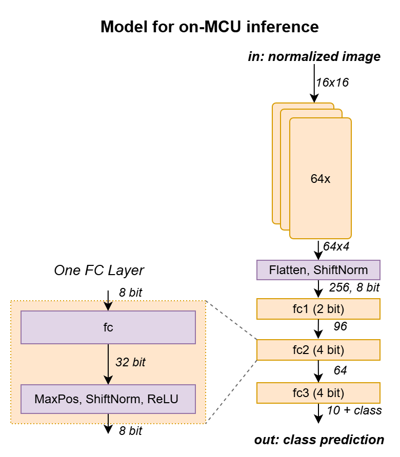
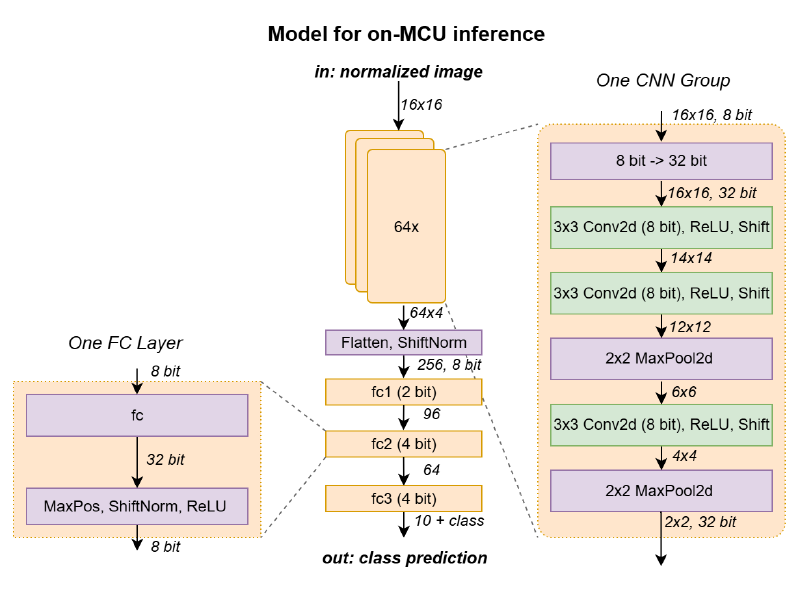
Following a lengthy “human-assisted architecture search,” I settled on the architecture below. The first layer of the former fully connected model is replaced with convolutional layers that perform the function of extracting features from the input image.
Sequential Depthwise Convolution and In-Place Processing#
The implementation of the CNN layers is somewhat unusual. Typically, a CNN is evaluated layer-by-layer. However, when the number of channels is expanded, this results in quickly increasing memory requirements. For example, to store the activations of a 16x16 image with 32-bit precision and 64 channels, we would need 16×16×4×64 B = 65,536 B = 64 kB of RAM, which far exceeds the capabilities of the target device. In addition, performing convolutions across all channels requires a lot of computational power—16×16×3×3×64×64 = 9,437,184 multiplications for just one layer.
To avoid this, a technique called depthwise separable convolutions has been introduced for architectures targeting mobile devices, prominently used in MobileNet4 and Xception5. Here, the convolution is split into two separate operations: a depthwise convolution that operates on each channel separately and a pointwise operation that combines the outputs. This reduces the number of parameters and computations significantly. For the example above, the number of multiplications reduces to 16×16×3×3×64 + 16×16×64×64 = 1,196,032, which is significantly less.
BitNetMCU applies this idea one step further with sequential depthwise convolutions and pooling per channel. Each channel is processed individually, and only the four final activations per channel are retained before combining them into the fully connected layers.
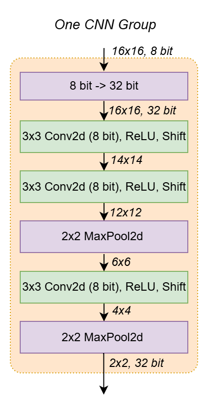
This approach enables in-place processing6, where the output of each layer replaces its input in the same memory region. The convolutions therefore only require the memory footprint of a single channel (1 kB for a 16×16 image stored in 32-bit integers).
Simplifying Convolutions and Implementation#
To further reduce complexity, the convolution is fixed to a 3×3 kernel with stride 1 and no padding. This avoids edge cases but risks missing patterns on the image boundary. Fortunately, MNIST rarely uses edge pixels, as shown below.
![]()
The code of the simplified convolution operation is shown below. It is unrolled for a 3×3 kernel and is fused with a ReLU activation function.
int32_t* processconv33ReLU(
    int32_t *activations,
    const int8_t *weights,
    uint32_t xy_input,
    uint32_t n_shift,
    int32_t *output
) {
    for (uint32_t i = 0; i < xy_input - 2; i++) {
        int32_t *row = activations + i * xy_input;
        for (uint32_t j = 0; j < xy_input - 2; j++) {
            int32_t sum = 0;
            int32_t *in = row++;

            // Unrolled convolution loop for 3x3 kernel
            sum += weights[0] * in[0] + weights[1] * in[1] + weights[2] * in[2];
            in += xy_input;
            sum += weights[3] * in[0] + weights[4] * in[1] + weights[5] * in[2];
            in += xy_input;
            sum += weights[6] * in[0] + weights[7] * in[1] + weights[8] * in[2];

            // Apply shift and ReLU
            if (sum < 0) {
                sum = 0;  // ReLU
            } else {
                sum = sum >> n_shift;
            }
            *output++ = (int32_t)sum;
        }
    }
    return output;
}
Variable Quantization#
The last piece of the puzzle was to use variable quantization. As shown in the full architecture diagram below, different quantization levels were used for weights and activations in different layers.
The convolutional layers turned out to be very sensitive to quantization. Notable degradation was even observed for 4-bit weights. Luckily, the number of weights in the convolution layers is rather small, so there is little memory benefit in quantizing to below 8 bits. Therefore, 8-bit quantization was used for the Conv2d layer weights.
However, the depthwise convolutions also turned out to be very sensitive to relative scaling errors in activations between the channels. In addition, to avoid mismatch between the channels, it was not possible to introduce normalization between the layers. I therefore opted to keep the activations in full 32-bit resolution and introduce fixed shifts to limit the dynamic range. Only after all channels are processed is normalization performed across all channels (layernorm). Subsequently, the activations are quantized to 8 bits before feeding the data into the fully connected layers.
   Layer (type)        Output Shape      Param #      BPW    Bytes #
========================================================================
    BitConv2d-1    [-1, 64, 14, 14]          576       8         576
    BitConv2d-3    [-1, 64, 12, 12]          576       8         576
    BitConv2d-6      [-1, 64, 4, 4]          576       8         576
   BitLinear-10            [-1, 96]       24,576       2       6,144
   BitLinear-12            [-1, 64]        6,144       4       3,072
   BitLinear-14            [-1, 10]          640       4         320
========================================================================
    Total                                 33,088              11,264
The first fully connected layer holds the most weights (256×96). Quantizing it to 2-bit weights saves memory and even improves performance slightly, likely due to regularization. The last two fully connected layers stay at 4-bit weights. Overall, the model consumes 11 kB of flash for weights, less than the fully connected model, leaving space for the extra inference code.
CNN Implementation Results#
Accuracy Trade-offs#
| Configuration | Width | BPW (fc1) | Epochs | Train Accuracy | Test Accuracy | Test Error | Model Size |
|---|---|---|---|---|---|---|---|
| 16-wide 2-bit | 16 | 2-bit | 60 | 98.43% | 99.06% | 0.94% | 5.4 kB |
| 32-wide 2-bit | 32 | 2-bit | 60 | 99.12% | 99.28% | 0.72% | 7.3 kB |
| 48-wide 2-bit | 48 | 2-bit | 60 | 99.30% | 99.44% | 0.56% | 9.3 kB |
| 64-wide 2-bit | 64 | 2-bit | 60 | 99.40% | 99.53% | 0.47% | 11.0 kB |
| 64-wide 4-bit | 64 | 4-bit | 60 | 99.41% | 99.44% | 0.56% | 12.3 kB |
| 64-wide 2-bit (90ep) | 64 | 2-bit | 90 | 99.47% | 99.55% | 0.45% | 11.0 kB |
| 80-wide 2-bit (90ep) | 80 | 2-bit | 90 | 99.51% | 99.42% | 0.58% | 13.2 kB |
The table above shows the results of different optimization and ablation experiments. Key findings are:
- Quantizing the first fully connected layer to 2 bits vs. 4 bits improves the test performance slightly, possibly due to better regularization. This result is reproducible. Even introducing dropout at various levels did not improve the performance of the 4-bit quantized model to that of the 2-bit model.
- Increasing the number of channels in the convolution layers improves train accuracy, as expected for a higher capacity model.
- The test accuracy is maximized for the 64-wide model and improves slightly with 90-epoch training.
The best result reached 99.55% test accuracy (0.45% error) with the 64-wide 2-bit model trained for 90 epochs—about a 0.5% improvement over the fully connected network while halving the test error.
Cross-validation between the quantized and exported 99.53% model produced only two mismatches between the Python and C inference engines, likely caused by numeric differences in normalization operations.
Verifying inference of quantized model in Python and C
  247 Mismatch between inference engines found. Prediction C: 6 Prediction Python: 2 True: 4
 3023 Mismatch between inference engines found. Prediction C: 8 Prediction Python: 5 True: 8
size of test data: 10000
Mispredictions C: 46 Py: 47
Overall accuracy C: 99.54 %
Overall accuracy Python: 99.53 %
Mismatches between engines: 2 (0.02%)
These results are notable, considering the constraints of using a 16×16 downsampled dataset, a strongly quantized model, and limitations in total weight size and available memory during inference.
The error rate is still among the state-of-the-art for CNN-based MNIST and qualifies for a top 100 position in the ongoing Kaggle leaderboards.
Pushing the model further proved difficult, as shown below. Walking further down the path of increasing model capacity by increasing the input width beyond 64 and using ternary weight quantization in fc1 for stronger regularization improved test loss but did not improve accuracy significantly. Experiments with further data augmentation (elastic distortions, random erasing) did not improve the test error.
| Configuration | Width | BPW (fc1) | Ep. | Train Acc. | Test Acc. | Test Error | Model Size |
|---|---|---|---|---|---|---|---|
| 64-wide 2-bit | 64 | 2-bit | 60 | 99.40% | 99.53% | 0.47% | 11.0 kB |
| 80-wide ternary | 80 | Ternary | 60 | 99.46% | 99.52% | 0.48% | 11.42 kB |
| 96-wide ternary | 96 | Ternary | 60 | 99.53% | 99.58% | 0.42% | 13.04 kB |
| 96-wide ternary (120 ep) | 96 | Ternary | 120 | 99.56% | 99.58% | 0.42% | 13.04 kB |
| 96-wide tern. + elastic | 96 | Ternary | 120 | 99.10% | 99.51% | 0.49% | 13.04 kB |
| 128-wide ternary | 128 | Ternary | 60 | 99.51% | 99.50% | 0.50% | 16.29 kB |
Additional experiments (not shown) with deeper fully connected layers, dropout, and 28×28 inputs did not meaningfully improve accuracy. Remaining errors appear to be out-of-distribution samples that would likely require either ensemble models or much larger models with different regularization schemes.
Performance on EMNIST Letters and Balanced#
The 64-wide CNN-96-64 model was also trained on the EMNIST_LETTERS and EMNIST_BALANCED datasets7, which contain more than 10 classes. Despite the model not being optimized for these more complex datasets, the performance is still very good.
| Dataset | Classes | Train Acc | Test Loss | Test Acc | Model Size (kB) |
|---|---|---|---|---|---|
| EMNIST_LETTERS | 37 | 93.63% | 0.172070 | 94.18% | 11.84 |
| EMNIST_BALANCED | 47 | 87.63% | 0.329145 | 88.24% | 12.17 |
The EMNIST_BALANCED dataset includes both numbers and letters, making it suitable for a simple OCR application on a low-end MCU.
Inference Performance on MCU#
Performance measurements were taken on a CH32V002 microcontroller running at 48 MHz with two flash wait states and inner loops executed from SRAM.
| Configuration | CNN Width | Size (kB) | Test Accuracy | Cycles Avg. | Time (ms) |
|---|---|---|---|---|---|
| 16-wide CNN, small fc | 16 | 3.2 | 98.92% | 686,490 | 14.30 |
| 16-wide CNN | 16 | 5.4 | 99.06% | 785,123 | 16.36 |
| 32-wide CNN | 32 | 7.3 | 99.28% | 1,434,667 | 29.89 |
| 48-wide CNN | 48 | 9.3 | 99.44% | 2,083,568 | 43.41 |
| 64-wide CNN | 64 | 11.0 | 99.55% | 2,736,250 | 57.01 |
| 1k 2Bitsym FC | - | 1.1 | 94.22% | 99,783 | 2.08 |
| 12k 4Bitsym FC | - | 12.3 | 99.02% | 528,377 | 11.01 |
| 12k FP130 FC | - | 12.3 | 98.86% | 481,624 | 10.03 |
Reducing the fully connected layers to 64/48 hidden units trims the parameter count substantially but barely shifts total inference time because the convolutional stages dominate runtime.
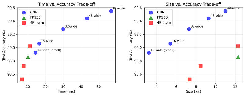
The plot above shows the trade-off between model size, accuracy, and inference time. CNN-based models clearly outperform in accuracy at the same parameter count. However, this comes at a steep increase in inference time.
Conclusion#
In conclusion, a very tedious manual architecture search allowed to identify a CNN architecture that achieves state-of-the-art MNIST accuracy on a low-end microcontroller with tight memory constraints, orders of magnitude smaller than typical models.
The key elements were the use of sequential depthwise convolutions with in-place processing, variable quantization, and simplified convolution operations. Regularization through strong quantization in the first fully connected layer played a crucial role in achieving high accuracy and is a topic worth further exploration.
The code can be found in the BitNetMCU GitHub repository.
References#
Y. LeCun et al. Gradient-based learning applied to document recognition (Proc. IEEE, 1998) ↩︎
D. Cireşan et al. Multi-column Deep Neural Networks for Image Classification (arXiv:1202.2745) ↩︎
A. Krizhevsky et al. ImageNet Classification with Deep Convolutional Neural Networks (NeurIPS 2012) ↩︎
A. G. Howard et al. MobileNets: Efficient Convolutional Neural Networks for Mobile Vision Applications (arXiv:1704.04861) ↩︎
F. Chollet. Xception: Deep Learning with Depthwise Separable Convolutions (arXiv:1610.02357) ↩︎
J. Lin et al. MCUNet: Tiny Deep Learning on IoT Devices (arXiv:2007.10319) ↩︎
G. Cohen et al. EMNIST: an extension of MNIST to handwritten letters (arXiv:1702.05373) ↩︎